The Maxwell School
Syracuse University
Syracuse University
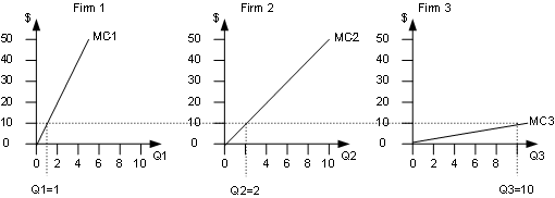
Graphing the curves:MC1 = 10*Q1
MC2 = 5*Q2
MC3 = 1*Q3.
For the cleanup to be done efficiently (that is, at minimum cost), we want to allocate the cleanup between the firms so that MC1 = MC2 = MC3. Since the three marginal costs will be equal, we can just write them as MC. Rewriting the equations above:
MC = 10*Q1
MC = 5*Q2
MC = 1*Q3.
Now rearrange each equation to show how much abatement each firm should do for any given choice of MC:
Q1 = MC/10
Q2 = MC/5
Q3 = MC
The total amount of abatement that will be done is the sum of these. Solving for it:
QT = Q1 + Q2 + Q3
QT = MC/10 + MC/5 + MC
QT = MC(1/10 + 2/10 + 10/10)
QT = (13/10)*MC
This gives the overall cost curve for pollution abatement when the cleanup is allocated efficiently across firms. It can also be rewritten:
MC = (10/13)*QT
Notice that the slope of the curve is smaller (the curve is flatter) than any of the individual marginal cost
curves. That's because we always get to pick the firm with the lowest abatement cost when choosing who should do
the next unit of abatement.
To see how this works, suppose we wanted to clean up 6 units of pollution and had to decide how to allocate it
between the sources. The table below shows the marginal cost of each unit of pollution abatement from each source:
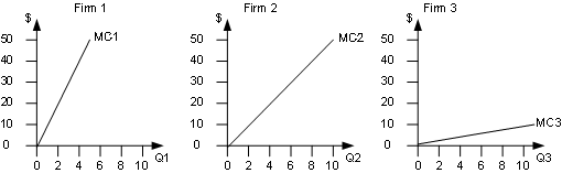
Q 1 2 3 4 5 6 7 8 9 10 MC1 10 20 30 40 50 60 70 80 90 100 MC2 5 10 15 20 25 30 35 40 45 50 MC3 1 2 3 4 5 6 7 8 9 10
The very first unit of pollution should be cleaned up by source 3 because its marginal cost is $1. The second
unit abated should also be cleaned up by source 3 because its cost is $2, which is still lower than the first unit
of abatement at either of the other sources. Following this logic, firm 3 should clean up all of the first five
units. The sixth unit of abatement, however, should be done by source 2. That's because its marginal cost is only
$5 while the cost of source 3 cleaning up an extra unit is $6. The six units are shown in green in the table.
At the seventh unit, clean up would switch back to source 3 until eleven total units had been abated. The twelfth
and thirteenth units, however, would be abated by sources 1 and 2. Units seven through thirteen are shown in yellow
in the table. As the amount of abatement increases, this pattern keeps repeating.
The efficient allocation of 13 units of abatement can be shown graphically as follows: